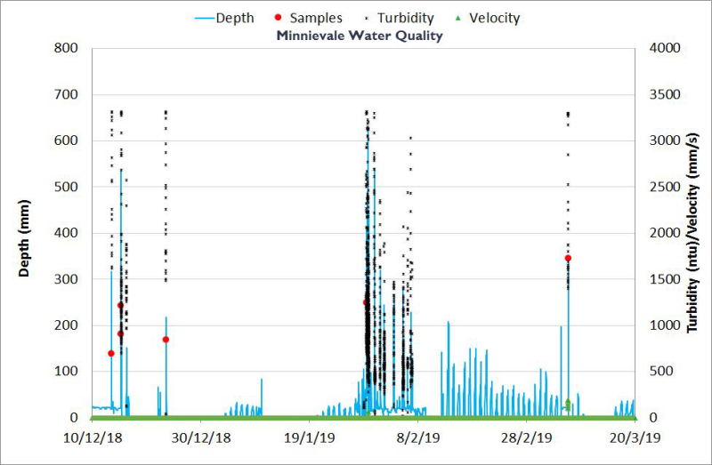
This dataset contains Water Quality monitoring data collected at the project gully sites for the three reporting wet seasons 2016-2017, 2017-2018 and 2018-2019. The data in presented in this metadata are part of a larger collection and are intended to be viewed in the context of the project. For further information on the project, view the parent metadata record: Demonstration and evaluation of gully remediation on downstream water quality and agricultural production in GBR rangelands (NESP TWQ 2.1.4, CSIRO). Monitoring of these sites is continuing as part of NESP TWQ Project 5.9. Any temporal extensions to this dataset will be linked to from this record. Methods: A description of the water quality sampling procedures for this project is outlined in Baker et al.,(2016). An automatic monitoring station was installed at each of the treatment gullies (See Key Localities). The monitoring station recorded rainfall, stage height, turbidity and water temperature at 1-min intervals during runoff events. The station also housed an ISCO auto-sampler that collected 1-L water samples at programmed intervals across the hydrograph (samples were processed as described below). A camera was installed at the treatment sites to capture photos during runoff events. Each of the control sites were fitted with a simpler tripod monitoring station that measured rainfall, stage height and turbidity. Bulk water quality samples were collected manually after each (accessible) event using poly-pipe rocket structures. Data from both the treatment and control sites had telemetered communications to allow remote access of data. Unidata Starflow QSD ultrasonic doppler was installed above the turbidity sensor at each site in 2017. The sensor measures the velocity of particles or bubbles in the water (presumed to be the same velocity as the water) using the doppler shift between transmitted and received ultrasonic signals. The sensors are mounted facing downstream to reduce the impact of particles damaging the sensor face and debris build up on measurement. The sensors require reconfiguration from factory default settings to capture data in gully systems. A description of the water quality sampling procedures for this project is outlined in Baker et al., (2016). In brief, following significant runoff events that triggered the samplers, the ISCO bottles were collected and the samples were filtered and frozen if collected within 24 hours of the event. These samples were analysed for TSS and the full suite of nutrients (total nitrogen, total dissolved nitrogen, NH3, NOx, total phosphorus, total dissolved phosphorus, FRP) at the JCU TropWater Laboratory, Townsville. Samples that were not collected within 24 hours were analysed for TSS only. A sub-set of the samples collected were also sent for particle size analysis. The samples were processed on a Malvern Mastersizer which is a laser diffraction analyser with a lens range of 0.02 – 2000 µm. Telemetered data from the loggers was captured to a fileserver and subsequently extracted, checked and combined with lab sample results in Excel. The files in this data collection represent the final combined dataset of all water quality and rainfall data from each site. Linear relationships between TSS and TN sample concentrations and coincident turbidity data were derived for all sites (Table 6). Turbidity data was not used when (i) the instrument exceeded the instrument calibration threshold; (ii) turbidity sensor readings were erroneous due to damage or sensor malfunction, or when the sensors were buried. Format: This data collection consists of 5 zip files (one for each paired gully monitoring site). Zip files are named according to the property on which they are located. Each zip file contains six MS Excel spreadsheets representing 3 years of water quality monitoring and rainfall data for both the Control and Treatment gully sites. MS Excel files contain tabs representing the following: Notes Rainfall Stream data (Timestamp, Depth, Turbidity, Rain, Photo cnt, Velocity) Sample Data (Timestamp, BottleNo, EventNo, SampleNo, Depth, Turbidity) Lab Results (combined with sample data) Chart of Stream and Sample data for the whole year and reporting Charts of Stream and Sample data for each flow event Each zip file contains an additional Excel spreadsheet “WQ_QA_vs_Turb_<site>.xlsx” with tabs “control” and “treatment” containing a summary of all water quality lab analyses for all years and an assessment of the quality (Quality_code) of each sample. Further tabs show the turbidity-TSS and turbidity-N relationships subsequently developed for use in discharge and load estimates. As well as the 5 zip files, this collection contains a single spreadsheet summarising all particle size measurements for the sites: “NESP_particle size_summary_all_sites.xlsx” Data Dictionary: Column headings used in the Water Quality Excel spreadsheets: Timestamp – time in AEST (+10GMT) Depth – Depth of flow above depth sensor in millimetres, Depth sensor was level with gully bed at time of installation. Turbidity – turbidity in units of NTU Velocity - Velocity is in units of mm/sec (note that the Turbidity and velocity sensors are mounted at between 100 and 400 mm above the depth sensor). Rain – rainfall in millimetres during period between current timestamp and previous timestamp PhotoCnt – site photo count value associated with timestamp BottleNo – Bottle number associated with ISCO sampler EventNo – Event number associated with sample SampleNo – Sample Number as submitted to Lab. Lab Results – headings are self-explanatory TSS = Total Suspended Sediment Column headings used in Particle_size sptreadsheet: Year – Wet season over which particle size sample was collected Event - indicator to allow for differentiation between events Site – site at whch samples awas collected (codes below) Date – sample collection date Sample number TSS – Total Suspended Sediment recorded in Stream data at sample timestamp <10 um - fraction of sample < 10 microns size Particle size - D10 - diameter (microns) at which 10% of the sample's mass is comprised of particles less than this diameter Particle size - D50 - diameter (microns) at which 50% of the sample's mass is comprised of particles less than this diameter Particle size - D90 - diameter (microns) at which 90% of the sample's mass is comprised of particles less than this diameter Source – the source of the data (name) if not CSIRO (Where D10,50,90 is the of < 10 micrometres). WQ_QA_vs_Turb_<site>.spreadsheets: “Treatment” and “Control” tabs contain Lab Results for all years at Treatment and Control gullies. An additional Quality_Code is used to assign a quality value to the Samples: 0 = good for tss/turb relationship & concentrations 1 = turbidity probe error - concentration data OK 2 = turbidity probe out of range - concentration data OK 3 = sample error (don’t use for concentrations) but turb data is OK The “TSS-Turb” and “N-Turb” contain the lab results used to derived the TSS-Turb and N-Turb relationships at each site. Site Codes used in filenames or Site columns are as follows: MIN = Minnievale MV = Meadowvale MW = Mount Wickham SB = Strathbogie VP = Virginia Park <T/C> - Treatment/Control Note: SBT is now the Strathbogie Control site SBC (to 2018) and SBT2 (after 2018) is now the Strathbogie Treatment site References: Baker, B., Hawdon, A. and Bartley, R., 2016. Gully remediation sites: water quality monitoring procedures, CSIRO Land and Water, Australia. Bartley, R., Hawdon, A., Henderson, A., Wilkinson, S., Goodwin, N., Abbott, B., Bake, B., Boadle, D., and Ahwang, K. (2019) Quantifying the effectiveness of gully remediation on off-site water quality: preliminary results from demonstration sites in the Burdekin catchment (third wet season). Report to the National Environmental Science Programme. Reef and Rainforest Research Centre Limited, Cairns (115 pp.). Data Location: This dataset is filed in the eAtlas enduring data repository at: data\NESP2\2.1.4-Gully-Remediation-effectiveness

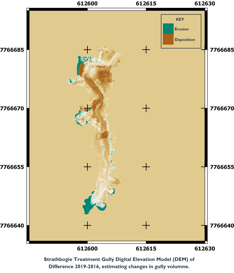
This dataset contains Riegl terrestrial laser scanner scans and their derived 5 cm gridded digital elevation models (DEMs) collected for up to 4 years between 2016 and 2019 for 4 paired Control/Treatment gully sites being monitored as part of NESP Project 2.1.4. Data collection also contains the DEMs of difference used to estimate changes in gully volume. The data in presented in this metadata are part of a larger collection and are intended to be viewed in the context of the project. For further information on the project, view the parent metadata record: Demonstration and evaluation of gully remediation on downstream water quality and agricultural production in GBR rangelands (NESP TWQ 2.1.4, CSIRO). Monitoring of these sites is continuing as part of NESP TWQ Project 5.9. Any temporal extensions to this dataset will be linked to from this record. Methods: Riegl terrestrial laser scanner (TLS) scans were collected for up to 5 years between 2015 to and 2019 for 4 paired Control/Treatment NESP gully sites. The fifth site, Mount Wickham, is not scanned. Each site was scanned once a year at the end of the wet season (generally April) using a Riegl terrestrial laser scanner. The TLS instrument used in this study was the RIEGL VZ400. The TLS was registered using five ground control points at each site. The control points consisted of a 50 cm star picket driven flush into the ground with a concrete collar. Survey bipods with reflectors were then placed over these marks to establish consistent xyz locations between scanners and for repeat surveys. To link RIEGL scans collected on the same day, additional ‘mobile’ reflectors were placed strategically around the sites. Registration was then performed by matching distances between reflector pairs (see Goodwin et al., 2016 for details). The RIEGL has an inbuilt fine-scan option to accurately locate reflector locations and is used to register separate scans into the same coordinate system with errors typically < 1 cm. These datasets are then projected into real world coordinates using the internal GPS and digital compass. The number of scans captured between sites varies due to differing morphological complexity and area to be mapped. Note that TLS scanning has not occurred at Mt Wickham. The georeferenced point clouds from each scan position are bundled as ZIP files by site and date. Naming conventions are explained in the data dictionary. The point clouds for each site and year were combined and converted into 5 cm digital elevation models (DEMs) by determining the minimum Z (elevation) value within a 5 cm grid pattern limited to an area covering the gully headcut and immediate downstream vicinity. A 3x3 grid cell median filter was used to remove spurious elevation values. Minimum Z is assumed to represent ground level. These DEMs are provided in TIFF format for each survey. Difference of DEMs (DoDs) were created by subtracting one DEM from another. Common extents were required for comparison of the DoDs. For the gully, a modified region grow approach was applied to an unclipped RIEGL DEM. This approach utilises a difference from mean elevation (DFME) (Evans and Lindsay, 2010) and a slope layer to detect the gully edges. A 50 cm buffer was then applied to ensure full capture of the gully edges. This dataset also includes hillshading derived from the DEMs. The original point cloud data is not available for download from the eAtlas (due to its large size), but is available on request from the Point of Contact. The DEMs are available for the following years and sites: Meadowvale: 2017, 2018, 2019 Minnievale: 2016, 2017, 2018, 2019 Strathbogie: 2016, 2017, 2018, 2019 Virginia Park: 2016, 2017, 2018, 2019 The DoDs correspond to the difference between the current year and the base year. Limitations of the data: Minimum Z DEM’s for representation of geomorphology ignore the possibility of overhangs. The raw DEMs provided include an area larger than the mapped gullies. These areas contain many anomalies as the scans were not intended to fully capture these areas. As a result the DEMs need to be masked before analysis is applied. Format: This dataset consists of multiple ZIP files containing LAZ files, ArcGIS shapefiles, JPGs and geoTIFF format grids Point_Clouds contains four folders, one for each paired Control/Treamenet gully monitoring site. Each folder contains Control and Treatment subfolders with zip files of the georeferenced TLS scans (as LAZ) by year. The file name convention is explained in the data dictionary. DEMs_and_DODs contains four ZIP files (one for each property) containing the DEMs and DEM of difference respectively in geoTIFF format at each control and treatment site for up to 5 years of monitoring between 2015 and 2019. File names For DEMs: <site>_<year>_DEM5cm.TIFF File names For Shaded relief DEMs: <site>_<year>_DEM5cm_HS.TIFF Where <site> is the 3 letter site code (see data dictionary) and <year> is the year surveyed (actual survey dates are captures in the naming convention of the Point Cloud files) NESP_2017_controlpoints_28355.shp contains the locations of the reference markers used for georeferencing the surveys. _META contains four zip files (one for each property) containing the DEMS and DODs in figures 21, 28, 36, and 44of the NESP report Bartley et al., 2019) All coordinates are GDA94 MGA zone 55. Data Dictionary: File naming convention for the Point clouds zip files (and LAZ files) <what>_<where>_<when>_<processing>[_optional][.suffix] <What> codes used: gp = ground platform v1 = Riegl VZ-400 dr = time-of-flight discrete return lidar <Where> - latitude longitude in decimal degrees <When> - YYYYMMDDTTTTTT <processing> ba3 = point clouds bc4 = Interpolated minimum heights to regular grid with median filtered applied m5 zone 55 The return deviation is stored in the ‘point_source_id’ field of the LAZ files and and the range is stored in the ‘GPS_time’ field. File naming Conventions for DEMs and DOD’s Site_Code used for file names are as follows: MIN = Minnievale MV = Meadowvale MW = Mount Wickham SB = Strathbogie VP = Virginia Park <T/C> - Treatment/Control Note: SBT is now the Strathbogie Control site SBC (to 2018) and SBT2 (after 2018) is now the Strathbogie Treatment site <year> = year measured DEM5cm = 5 cm gridded digital elevation model of ground surface DEM5cm_HS = hillshade of DEM DoD_<year2>-<year1> = DEM of difference Mask = mask showing extents used for DoD References: Bartley, R., Hawdon, A., Henderson, A., Wilkinson, S., Goodwin, N., Abbott, B., Bake, B., Boadle, D., and Ahwang, K. (2019) Quantifying the effectiveness of gully remediation on off-site water quality: preliminary results from demonstration sites in the Burdekin catchment (third wet season). Report to the National Environmental Science Programme. Reef and Rainforest Research Centre Limited, Cairns (115 pp.). Bartley, R., Goodwin, N., Henderson, A.E., Hawdon, A., Tindall, D., Wilkinson, S.N. and Baker, B., 2016. A comparison of tools for monitoring and evaluating channel change, Project 1.2b. Report to the National Environmental Science Programme. Reef and Rainforest Research Centre Limited, Cairns (36pp.). NR Goodwin, J Armston, I Stiller, J Muir. (2016) Assessing the repeatability of terrestrial laser scanning for monitoring gully topography: A case study from Aratula, Queensland, Australia, Geomorphology 262, 24-36. Data Location: This dataset is filed in the eAtlas enduring data repository at: data\NESP2\2.1.4_Gully_Remediation_Effectiveness

This dataset contains Vegetation and Biomass monitoring data collected for the NESP TWQ Project 5.9, formally NESP TWQ 2.1.4 - Demonstration and evaluation of gully remediation on downstream water quality and agricultural production in GBR rangelands and Landholders Driving Change (LDC) contracts LRP17-003 and LME17-009. Data is from control and treatment gully sites on commercial grazing properties in the Burdekin. BOTANAL files describe the biomass, species composition and species attributes such as basal area and cover for hillslope areas above gully erosion sites. PATCHKEY files describe the landscape condition (proportional) of vegetation patches for hillslope areas above gully erosion sites. GULLY_VEG describes the biomass, species composition and species attributes such as percent cover for locations within the Gully. Seven paired Control/Treatment gully sites on commercial grazing properties in the Burdekin being monitored as part of NESP Project 5.9 and NESP Project 2.1.4 (Demonstration and evaluation of gully remediation on downstream water quality and agricultural production in GBR rangelands) and Landholders Driving Change (LDC) contracts LRP17-003 and LME17-009. The key question being asked is "is there measureable improvement in the erosion and water quality leaving remediated gully sites compared to sites left untreated?" The monitoring approach uses a modified BACI (Before after control impact) design. The aim of the vegetation monitoring in relation to this project is to track change in land condition and vegetation over time on hillslope areas above, and within gullies within control and treatment sites (treatments vary). Linking to changes in downstream water quality. Methods: Vegetation metrics were measured on the hillslope above and within each of the monitored gullies at the Pre-wet or end of the dry season ('EOD', October–November) and then again at the post-wet or end of the wet season ('EOW', April). Measurements were initiated in November 2016 at all sites except Mt Wickham which started in August 2018 and at Mt Pleasant and Glen Bowen that began in November 2019. For BOTANAL and PATCHKEY, Landscape and vegetation condition transects were installed upslope of the uppermost head section on both the treated and control gullies at all sites. Transects were run along slope contours and varied in length and spacing for each site depending on gully-head catchment size. Four to five transects were used at each treatment and control location. Each transect has a fixed beginning and end to facilitate repeat measures. Length and spacing of transects varied between sites dependant on hillslope size. 6 to 8 x 1m quadrats were sampled along each transect at equal spacing giving 30 to 32 samples per site (this may vary due to some changes in study sites over time – eg. New fence placements or inaccessibility due to weather). See "Interactive map of this dataset" in the online resources for layouts at sites. BOTANAL data was collected along each transect using a 1m² quadrat using the methods of Tothill et al., (1992), with placement of quadrats dependent on transect length at each site (30 quadrats were sampled for each treatment/control area). Metrics included the main pasture species and/or functional group composition and frequency, above-ground pasture biomass (DMY), total cover, litter cover, basal-area %, defoliation level and key soil surface condition metrics (Tongway and Hindley, 1995). In addition landscape condition was calculated along each transect using PATCHKEY (Abbott and Corfield, 2012). The condition assessments were aggregated to reflect ABCD landscape condition as used across grazed landscapes in the GBR catchments (Aisthorp and Paton, 2004; Chilcott et al., 2005; Bartley et al., 2014). Cover and biomass estimates were calibrated against standard quadrats taken at each site using classified quadrat photographs. Biomass standards were oven dried to attain dry matter yield, removing vegetation water retention error between treatments. A real time kinematic (RTK) survey ran from upslope of the vegetation survey to the valley section for each gully system. Data was collected at 4 to 5 parallel fixed transects above gully locations (hillslope area) – length and spacing of transects varied between sites dependant on hillslope size. See "Interactive map of this dataset" in the online resources for transect locations at sites. PATCHKEY data was collected digitally using custom software on handheld android devices. Survey occurred each year before and after wet season. Biomass is calibrated against cut and dried samples and cover is calibrated against classified quadrat photos – per collector. GULLY_VEGetation cover and biomass were also measured within each gully, on the gully walls and gully floor. Sampling was initiated at the end of the first wet season (April 2017) for all sites except Mt Wickham which started in August 2018 and at Mt Pleasant and Glen Bowen that began in November 2019. The sampling methodology was very similar to the hillslope survey. A minimum of three transects were measured across each gully, representative of the head, middle and valley sections. At each transect, % cover, biomass and dominant cover type was assessed using 0.25 m² (0.5 x 0.5m) quadrats. Three quadrats were assessed on each wall (six in total) and six quadrats assessed in the deepest part of the channel in the gully floor. Box plots of the % cover and biomass data at the end of each wet season for control and treatment sites were analysed using Sigmaplot Version 14. In most cases a t-test for means and non-parametric Mann-Whitney rank sum test were conducted to evaluate differences between treatment and control sites. Limitations of the data: This dataset contains Vegetation monitoring data collected at these gully sites for Pre-wet or end of the dry season ('EOD', October–November) for Hillslope only and then again post-wet of end of the wet season ('EOW', April) for Hillslope and Gully over four reporting periods 2016-2017, 2017-2018, 2018-2019 and 2019-2020. Measurements were initiated in November (EOD) 2016 at all sites except Mt Wickham which started in August (EOD) 2018 and at Mt Pleasant and Glen Bowen that began in November 2019. Format: This data collection consists of 4 zip files. BOTANAL.zip contains eight CSVs containing pre-wet and post-wet survey data for all sites for dates between 2016 and 2020. In addition there is a species (SPP) decode CSV. PATCHKEY.zip contains eight CSVs containing pre-wet and post-wet survey data for all sites for dates between 2016 and 2020. GULLY_VEG.zip contains 4 XLSX files containing post-wet gully vegetation survey data for all sites for dates between 2016 and 2020. Post-Wet end of wet (EOW). Individual tabs for each site record the raw data as captured in the field. The "Stds" tab calculated the calibration from BIO code to actual biomass. The "all_for_stats" sheet (or "All End of Wet" in file "Gully_Veg_2017-2018.xlsx") is the intermediate sheet for collation of data in "Wall" and "Channel" sheets ready for analysis in stats package. "Summary" tab contains summary data for the report. Veg_Spatial.zip consists of three shapefiles, Veg_transect_Locations.shp and Veg_Quadrat_locations.shp contain the transects and quadrat locations respectively in MGA94 Z55 coordinates for the BOTANAL and PATCHKEY surveys. Gully_Veg_locations.shp contains locations of the GULLY_VEG gully vegetation surveys in EPSG:4326 coordinates. Data Dictionary: Site Codes are as follows: - MIN = Minnievale - MV = Meadowvale - MW = Mount Wickham - SB = Strathbogie - VP = Virginia Park - MTP = Mount Pleasant - GLB = Glen Bowen <T/C> - Treatment/Control Note: Original Strathbogie control sites exhibited very high erosion rates and treatment was undertaken in Oct/Nov 2019 to stabilise. The treatment site "SBT" became the control site and the site ID was changed for "SBT (C)". Similarly, the control site "SBC" became the treatment site and the site ID was changed to "SBC / SBT2 (T)". Sites names were standardised for all data files except the GULLY_VEG.ZIP files. If you need more information, please contact Dr Rebecca Bartley. BOTANAL CSV headers: - ID: Unique identifier for sample - USER: Collector name/initials - SITE: Abbreviated site name - Meadowvale (MedV), Minnivale (MinV), Virginia Park (VP), Strathbogie (SB) and Mt Wickham (Mt W). Abbreviations are followed by a C for control site and T for treatment site – eg. MedVC, MedVT. - TRAN: Transect number, numbered from nearest to gully head – see attached GIS layer "Sites_transect and quadrat.shp.zip" - QUAD: Quadrat number per transect - see attached GIS layer "SIte_quadrat_locations.shp" - DATE: Date and time - SP1 to SP5: Species name abbreviated using first two letters of genus and first three of species name eg. Bothriochloa pertusa = boper. Species usually recorded in order of highest biomass represented. See "BOTANAL_Spp_decode.csv" for decode of species codes. - SPP1 to SPP5: Species proportion (%) estimate by biomass of quadrat for each of species 1 to 5 - YIELD: Total biomass estimate for quadrat in kg/ha - DEFOL: Estimated grazing defoliation of the pasture within a quadrat. Ordinal – 1=0-5%, 2=5-25%, 3=25-50%, 4=50-75% and 5=75-100% - BASAL: Estimated basal area of Perennial tussock grasses. % of quad - COVER: Foliage projected cover of pasture species, % of quad - LITTER: Litter cover, % of quad - BARE: Bare ground, % of quad (optional – usually the inverse of total cover ) - HARD: Soil hardness (scaled after Tongway et al 2004 – landscape functional analysis). Categorical – 1=Easily broken, 2=Moderately hard, 3=Very hard, 4=Sand, 5=Self mulching. - DEPOS: Deposition from erosion processes, (scaled after Tongway et al 2004 – landscape functional analysis) Categorical – 1=Insignificant, 2=slight, 3=moderate, 4=extensive - INCORP: Litter incorporation into soil surface. (scaled after Tongway et al 2004 – landscape functional analysis) Categorical – 1=nil, 2=low, 3= moderate, 4=high - EROSION: (scaled after Tongway et al 2004 – landscape functional analysis) Categorical – 1=Insignificant, 2=slight, 3=moderate, 4=extensive. PATCHKEY CSV Headers: - ID: Unique identifier for sample - DATE: Date and time - RECORDER: Collector name/initials - SITE: Abbreviated site name - Meadowvale (MedV), Minnivale (MinV), Virginia Park (VP), Strathbogie (SB) and Mt Wickham (Mt W). Abbreviations are followed by a C for control site and T for treatment site – eg. MedVC, MedV. - TRAN: Transect number, numbered from nearest to gully head – see attached GIS layer "Sites_transect and quadrat.shp.zip" - PATCH_NO: Number of the patch occurring along a transect – patches can be measured from either end of the transect. - DOMINANT: Dominant vegetation functional group within a patch. 3P=Native decreaser perennial tussock grasses, INPG=Native increaser perennial tussock grasses, EXPGT=Exotic perennial tussock grasses, EXPGS=Exotic perennial stoloniferous grasses (eg. Indian couch), ANNG=Annual grasses and forbs, SHRUBS=Shrubs less than 2m, BARE=Bare earth. - BASAL: Estimated basal area of Perennial tussock grasses. % of patch - LITTER: Litter cover. % of patch - YIELD: Total biomass estimate for patch in kg/ha - BARE: Bare ground % of patch - EROSION: Erosion severity (scaled after Tongway et al 2004 – landscape functional analysis ) Categorical – 1=Insignificant, 2=slight, 3=moderate, 4=extensive - HARDNESS: Soil hardness (scaled after Tongway et al 2004 – landscape functional analysis). Categorical – 1=Easily broken, 2=Moderately hard, 3=Very hard, 4=Sand, 5=Self mulching. - INCORPORATION: Litter incorporation into soil surface. (scaled after Tongway et al 2004 – landscape functional analysis) Categorical – 1=nil, 2=low, 3= moderate, 4=high - PATCH_TYPE: Patch type condition classification auto-calculated in software from the above inputs - PATCH_EST: Patch type condition estimated by user – overrides calculated value if required - PATCH_LENGTH: Measured patch length along transect Gully_Veg XLSX spreadsheets: Spreadsheets contain tabs for each gully site with fields as follows: - Date: date of measurement - Quad: quadrat measured (not always numbered) - Loc: location on gully –cross sections from RTK. Numbers are in order from 1 nearest incrementing by 1 downstream - Pos: walls (left bank (lb), right bank (rb)) or channel - BIO: biomass code from 0 to 5 – this is a surveyor-specific estimate which is calibrated to actual biomass using standards - Cov: estimate of percent cover - Sp: species composition. Please, contact Dr Rebecca Bartley for information regarding species codes. - COMMENT: any comments relating to the quadrat or measurement - Biomass (kg/ha): biomass calculated using standards - Surveyor: surveyor number (different standards calibration required for different surveyors) Each Gully_veg spreadsheet also contains additional tabs for calibration or summarising the survey data. - stds: contains calibration data for biomass estimation from Biomass codes. - Summary: summary statistics by site and location - All for Stats: an intermediate sheet used for deriving summary statistics - Channel: an intermediate sheet used for deriving summary statistics - Walls: an intermediate sheet used for deriving summary statistics - Instructions: Instructions for user Gull_Veg_locations FIELDNAMES: - Gully: Gully site code - Survey: "gully" for linear gully geometry or "alluvial Gully" for alluvial gully geometry - Location: Survey location for corss-referencing with Gully_Veg.XLSX sheets - POINT_X: Easting (m) in MGA94 UTM coordinates - POINT_Y: Northing (m) in MGA94 UTM coordinates Veg_transect_Locations.shp FIELDNAMES: - TRANSECT: transect number - SITE: site code Veg_Quatrat_Locations.shp FIELDNAMES: - TRANSECT: transect number - QUADRAT: quadrat number - SITE: site code - POINT_X: Easting (m) in MGA94 UTM coordinates - POINT_Y: Northing (m) in MGA94 UTM coordinates References: Bartley, R., Hawdon, A., Henderson, A., Abbott, B., Wilkinson, S., Goodwin, N. and Ahwang, K. (2020). Quantifying the effectiveness of gully rehabilitation on off-site water quality: results from demonstration sites in the Burdekin catchment (2019/20 wet season). Report to the National Environmental Science Programme. Reef and Rainforest Research Centre Limited, Cairns (138 pp.). Baker, B., Hawdon, A. and Bartley, R., 2016. Gully remediation sites: water quality monitoring procedures, CSIRO Land and Water, Australia. Abbott BN and Corfield JP (2012) PATCHKEY – A patch based land condition framework for rangeland assessment and monitoring, BACKGROUND INFORMATION AND USERS GUIDE. CSIRO, Australia. Tothill, J. C., et al. (1978). 1, BOTANAL - a comprehensive sampling and computing procedure for estimating pasture yield and composition. 1. Field sampling., CSIRO Division of Tropical Crops and Pastures. Tongway, D. J. and N. L. Hindley (2004). Landscape Function Analysis Manual: Procedures for Monitoring and Assessing Landscapes with Special Reference to Minesites and Rangelands. Ver. 3. 1. Canberra, CSIRO Review notes: the eAtlas reviewed this record on 12/09/2023 and updated the title of the record to be more descriptive of the project and in line with other records published in the series [formerly titled Gully remediation effectiveness - Vegetation 2019 - 2020 (NESP TWQ 5.9, CSIRO)". Other minor changes included updating a grammatical error in the abstract, and adding the linked resource for Vegetation Surveys of Sites for Gully Remediation (NESP TWQ 2.1.4, CSIRO). Data Location: This dataset is filed in the eAtlas enduring data repository at: data\custodian\2019-2022-NESP-TWQ-5\5.9_Gully-remediation-effectiveness-vegetation

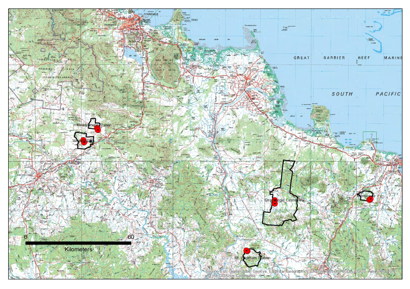
Five paired Control/Treatment gully sites on commercial grazing properties in the Upper Burdekin and Bowen catchments are being monitored as part of NESP Project 2.1.4 (Demonstration and evaluation of gully remediation on downstream water quality and agricultural production in GBR rangelands) (Bartley et al., 2018). The key question being asked is: "Is there measurable improvement in the erosion and water quality leaving remediated gully sites compared to sites left untreated?" The monitoring approach uses a modified BACI (Before after control impact) design. This record acts as an aggregation point for the datasets produced by NESP TWQ Project 2.1.4. for Gully Remediation at sites Meadowvale, Virginia Park, Strathbogie, Minnievale and Mt Wickham Station. These sites are located in the Burdekin Region of Queensland. The time series established in this project is being extended by NESP TWQ Project 5.9. Updated versions of this dataset will be linked to from this record when they become available. There are two sites in the Upper Burdekin sites (Virginia Park and Meadowvale) which capitalize on previous research investments looking at rangeland management and water quality response. The Bogie (Strathbogie) and Don (Minnievale) sites are Reef Trust 2 partnership projects. Mt Wickham is a new site that is part of the Burdekin Landholders Driving Change (LDC) project. Each contributing datasets has been described in specific dataset records linked as child records. Datasets include Key Localities, Loads Runoff, Site Configuration and survey types, TLS Scans and Analysis, Vegetation Survey, Water Quality survey. The data can be downloaded from each of the child records.

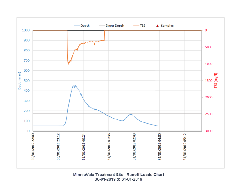
This dataset contains preliminary estimates of discharge and loads (Total suspended sediment and total nitrogen) based on monitoring data collected for the NESP Project 2.1.4 Demonstration and evaluation of gully remediation on downstream water quality and agricultural production in GBR rangelands. The data in presented in this metadata are part of a larger collection and are intended to be viewed in the context of the project. For further information on the project, view the parent metadata record: Demonstration and evaluation of gully remediation on downstream water quality and agricultural production in GBR rangelands (NESP TWQ 2.1.4, CSIRO). Monitoring of these sites is continuing as part of NESP TWQ Project 5.9. Any temporal extensions to this dataset will be linked to from this record. Methods: To estimate loads of suspended sediment (TSS) and total nitrogen (TN) the following steps were undertaken: (1) Depth, velocity and RTK surveyed cross-sectional area data were used to generate a stage-discharge rating curve for each site; (2) Linear relationships between TSS and TN sample concentrations and coincident turbidity data were derived for all sites (Table 6). Turbidity data was not used when (i) the instrument exceeded the instrument calibration threshold; (ii) turbidity sensor readings were erroneous due to damage or sensor malfunction, or when the sensors were buried. These relationships allowed for estimation of TSS and N from turbidity. When there was no turbidity data (due to sensor issues or instrument burial), TSS and TN concentrations were infilled using sample interpolation. (3) Total suspended sediment (TSS) and total nitrogen (TN) loads were then generated for each event and each water year (generally Nov to April) by multiplying discharge by concentration. (4) For all sites flow weighted annual average mean concentrations (FWAAC) were generated by dividing the annual load by annual runoff. This provided a quick visual assessment of the relative change in concentration between sites. (5) For some sites (i.e. Mt Wickham) event mean concentrations (EMCs) were generated for individual events by dividing the event load by event runoff. This provided a flow weighted mean concentration for each event. The event mean concentration (EMC) value for each event and year was calculated using mass of the sediment (in tonnes) divided by the runoff volume (in ML) during the time interval (T) (after Kim et al., 2004). Limitations of the Data: This dataset contains Water Quality monitoring data collected at these gully sites for the three reporting wet seasons spanning June-July 2016-2017, 2017-2018 and 2018-2019. During this study, the project had challenges with (i) sensor malfunctions (ii) sensor burial and re-scour (iii) sensors being damaged by moving objects (iv) green ant nests in sensors and (v) wires chewed by livestock. In addition sampling error or uncertainty in the discharge and load calculations can be high in semi-arid systems (Kuhnert et al., 2012). Consequently, all runoff and loads estimates are considered preliminary and will likely change in subsequent reporting years. Format: This data collection consists of 5 zip files (one for each paired gully monitoring site). Zip files are named according to the property on which they are located. Each zip file contains eight to twelve MS Excel spreadsheets representing daily and annual discharge and load estimates for both the Control and Treatment gully sites. MS Excel files contain tabs representing the following: SETUP – contains the site specific parameters used to estimate discharge and loads such as catchment size, location of instruments relative to depth sensor or gully cross section, discharge rating curve, and constituent-turbidity relationship SUMMARY – provides annual totals for rainfall, runoff, and loads, daily rainfall runoff chart, summary tables of rainfall and runoff events. RUNOFF_LOADS_CHART – chart of timeseries of depth, event depth, TSS or N concentration (as estimate from turbidity) and sample concentration - used to check for issues with depth or turbidity when interpreting annual or daily totals DAILY_SUMMARY_ALL_DATES – for generating daily rainfall, runoff and load estimates SAMPLES – list of sample values relevant to loads sheet period for cross checking against turbidity relationship RUNOFF LADS CALCS ALL TIMESTEP - raw Stream data with associated instantaneous calculations of discharge and loads RAIN AT GAUGE – rainfall timeseries from site (or closest) gauge RAIN USED FOR AVERAGING – if catchment is large, a second rain gauge may be used for averaging (not usually for gullies) Data Dictionary: Column headings used in the Excel spreadsheets: Timestamp – time in AEST (+10GMT) Depth – Depth of flow above depth sensor in millimetres, Depth sensor was level with gully bed at time of installation. Turbidity or Turb – turbidity in units of NTU (note that the Turbidity and velocity sensors are mounted above the depth sensor by 100 mm or more). Rainfall – rainfall in millimetres Discharge – discharge as either a rate or a total volume of water Runoff – discharge divided by catchment area Sample – Sample Number as submitted to Lab TSS / N = Total Suspended Sediment / Total Nitrogen Site_Code used for file names is as follows: MIV = Minnievale MV = Meadowvale MW = Mount Wickham SB = Strathbogie VP = Virginia Park <T/C> - Treatment/Control Note: SBT is now the Strathbogie Control site SBC (to 2018) and SBT2 (after 2018) is now the Strathbogie Treatment site References: Bartley, Rebecca; Hawdon, Aaron; Henderson, Anne; Wilkinson, Scott; Goodwin, Nicholas; Abbott, Brett; Baker, Brett; Matthews, Mel; Boadle, David; Jarihani, Ben (Abdollah). (2018) Quantifying the effectiveness of gully remediation on off-site water quality: preliminary results from demonstration sites in the Burdekin catchment (second wet season). RRRC: NESP and CSIRO. csiro:EP184204. Baker, B., Hawdon, A. and Bartley, R., 2016. Gully remediation sites: water quality monitoring procedures, CSIRO Land and Water, Australia. eAtlas Visualisation The visualisation presented on the eAtlas maps is a derived product of the summary data found within this data collection. A summary dataset was created using information presented on each spreadsheet [Water-Year, Site, Catchment Area, Rainfall, Runoff, %Runoff, Total TSS Load, Average TSS from time series, Total N Yield, N Loss, Average B from timeseries]. Two additional columns were added to the core information: data infill as referenced in the spreadsheets, has been represented in column 'Contains_Infilled_Data' noting Y or N; column 'Treatment_Control' was added to the summary dataset to aid visual representation, where treatment 'T' and control 'C' sites clearly identified. Data Location: This dataset is filed in the eAtlas enduring data repository at: data\nesp2\2.1.4_Gully-remediation-effectiveness

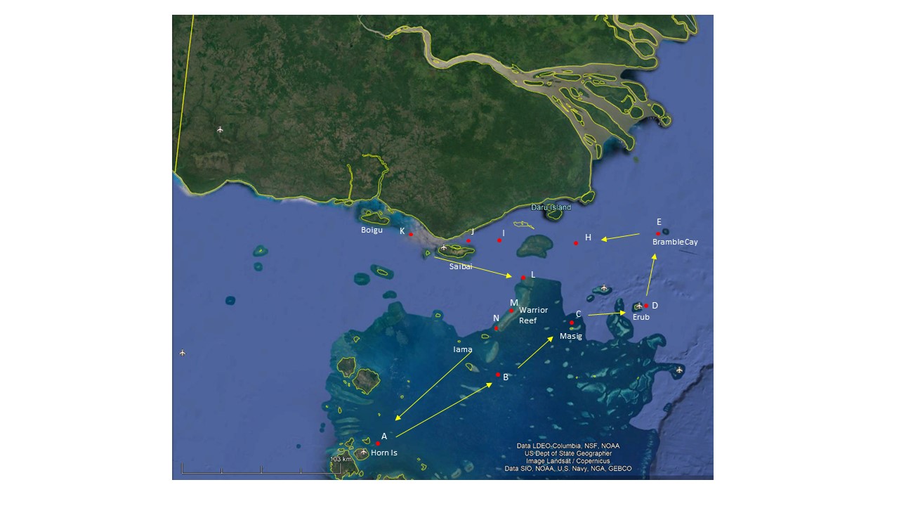
The data set comprises 4 spreadsheets containing trace metal concentrations measured in waters benthic, suspended sediments and seagrasses collected across the Torres Strait during the NESP TWQ 5.14 project. Details of the sampling locations (including coordinates), general chemical and physical parameters and laboratory quality control data are provided. The seagrass data set is also supported by historical data from previous studies: Dight, I.J., Gladstone, W. (1993). Torres Strait baseline study: pilot study final report June 1993. Great Barrier Reef Marine Park Authority Research Publication No. 29. Townsville, Great Barrier Reef Marine Park Authority and Waterhouse, J., Petus, C., Bainbridge, S., Birrer, S.C., Brodie, J., Chariton, A.C., Dafforn, K.A., Johnson, J.E., Johnston, E.L., Li, Y., Lough, J., Martins, F., O’Brien, D., Tracey, D., Wolanski, E., (2018). Identifying the water quality and ecosystem health threats to the Torres Strait and Far Northern Great Barrier Reef arising from runoff of the Fly River. Report to the National Environmental Science Programme. Reef and Rainforest Research Centre Limited, Cairns, 157 pages. The overall aim of the project is to identify the fate of waters from the Fly River in Papua New Guinea and their potential impact on the Torres Strait region. These data sets are metal concentrations in waters, sediments, and seagrasses from locations in the Torres Strait. Some background knowledge of environmental chemistry and water quality management in Australia is needed to properly interpret this data. Methods: Full details of sample collection, chemical analysis, and data processing are provided in the NESP report: Waterhouse, J., Apte, S.C., Petus, C., Angel, B.M., Wolanski, E., Bainbridge, S., Tracey, D., Jarolimek, C.V., King, J., Mellors, J., Brodie, J., (2021). NESP Project 5.14. Assessing the influence of the Fly River discharge on the Torres Strait. Report to the National Environmental Science Programme. Reef and Rainforest Research Centre Limited, Cairns. In brief: - Water samples were collected at locations around Boigu and Saibai (see maps in spreadsheets for details). - Sediment cores were collected using a gravity corer at locations detailed in the spreadsheets and sectioned in the field. The samples were frozen and transported to CSIRO Lucas Heights for analysis. - Seagrass samples were either, taken by hand or seagrass rake (5 replicates), transferred to ziplock plastic bags and stored frozen and then transported to the CSIRO Lucas Heights Laboratory for trace metal analysis. - Water samples were filtered, metals extracted and determined by inductively coupled plasma mass spectrometry. - Sediment samples were digested in mixed acids using microwave assisted dissolution and determined by inductively coupled plasma mass spectrometry. - Sediment was rinsed from the seagrass leaves with Milli-Q® water before a minimum of 200 mg of seagrass was weighed for each sample. The seagrass was then freeze dried using a Christ Alpha 1-2 LD Freeze Dryer. The dried seagrass samples were digested by high pressure/temperature nitric acid microwave digestion using a CEM MARS6 Microwave (in-house Method C-225). Metals were quantified by Inductively coupled plasma mass spectrometry (ICP-MS) using an Agilent 8800 ICP-MS (in-house method C-209). The certified reference material BCR-279 (Sea Lettuce, Ulva Lactua) was digested and analysed with the samples as a check on accuracy. Limitations of the data: The data provided presents a snapshot of water, sediment and seagrass quality at locations in the Torres Strait. It is not a comprehensive data set in terms of spatial and temporal coverage. Guidelines have not yet been developed to identify environmentally acceptable ranges of trace element concentrations for seagrass. Many factors can affect metal concentrations measured. Factors can include sampling intensity, timing of sampling, analytical procedures; relative concentration of other metals in the plant and the surrounding environment; as well as the species, part, and age of plant analysed. Consequently, any comparisons or conclusions between studies should be made with caution. Format: The data set comprises four Excel spreadsheets: - "NESP 5.14 Dissolved metals data.xlsx" - "NESP 5.14 Metals in benthic sediments.xlsx" - "NESP 5.14 Metals in suspended sediments.xlsx" - "NESP 5.14 eAtlas NESP 5.14 seagrass submission.xlsx" Important note: Tabs are also provided in the spreadsheet to show the data from the 2016 and 1991 Torres Strait Baseline Study for reference – however, these were obviously not collected as part of Project 5.14. References: Waterhouse, J., Apte, S.C., Petus, C., Angel, B.M., Wolanski, E., Bainbridge, S., Tracey, D., Jarolimek, C.V., King, J., Mellors, J., Brodie, J., (2021). NESP Project 5.14. Assessing the influence of the Fly River discharge on the Torres Strait. Report to the National Environmental Science Programme. Reef and Rainforest Research Centre Limited, Cairns. Waterhouse, J., Petus, C., Brodie, J., Bainbridge, S., Wolanski, E., Dafforn, K.A., Birrer, S.C., Lough, J., Tracey, D., Johnson, J.E., Chariton, A.C., Johnston, E.L., Li, Y., Martins, F., O’Brien, D. (2018) Identifying water quality and ecosystem health threats to the Torres Strait and Far Northern GBR from runoff of the Fly River. Report to the National Environmental Science Program. Reef and Rainforest Research Centre Limited, Cairns (162pp.). Dight, I.J., Gladstone, W. (1993). Torres Strait baseline study: Pilot study final report June 1993. Great Barrier Reef Marine Park Authority Research Publication No. 29. Townsville, Great Barrier Reef Marine Park Authority. Restrictions on raw data: Data set owners and TSRA rangers should be acknowledged for the data collection. Data Location: This dataset is filed in the eAtlas enduring data repository at: data\custodian\2019-2022-NESP-TWQ-5\5.14_TS-water-quality

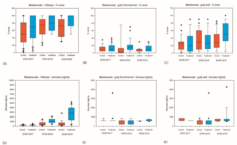
This dataset contains Vegetation and Biomass monitoring data collected for the NESP Project 2.1.4 (Demonstration and evaluation of gully remediation on downstream water quality and agricultural production in GBR rangelands). The aim of the vegetation monitoring in relation to this project is to track change in biomass and species composition over time on hillslope areas above gully erosion within control and treatment sites (treatments vary), linking to changes in downstream water quality. Data is from control and treatment gully sites on commercial grazing properties in the Burdekin being monitored as part of NESP Project 2.1.4. The data in presented in this metadata are part of a larger collection and are intended to be viewed in the context of the project. For further information on the project, view the parent metadata record: Demonstration and evaluation of gully remediation on downstream water quality and agricultural production in GBR rangelands (NESP TWQ 2.1.4, CSIRO) Monitoring of these sites is continuing as part of NESP TWQ Project 5.9. Any temporal extensions to this dataset will be linked to from this record. BOTANAL files describe the biomass, species composition and species attributes such as basal area and cover for hillslope areas above gully erosion sites. PATCHKEY files describe the landscape condition (proportional) of vegetation patches for hillslope areas above gully erosion sites. And BIOMASS files describe the cover and biomass within the gully. Methods: Vegetation metrics were measured on the hillslope above each of the NESP gullies at the end of the dry season (‘EOD’, October–November) and then again at the end of the wet season (‘EOW’, April). Measurements were initiated in November 2016 at all sites except Mt Wickham which started in August 2018. Landscape and vegetation condition transects were installed upslope of the uppermost head section on both the treated and control gullies at all sites (Figure 8). Transects were run along slope contours and varied in length and spacing for each site depending on gully-head catchment size. Four to five transects were used at each treatment and control location. Each transect has a permanent marker at the beginning and end to facilitate repeat measures. Pasture metrics were recorded along each transect using a 1m2 quadrat based on the methods of Tothill et al., (1992), with placement of quadrats dependent on transect length at each site (30 quadrats were sampled for each treatment/control area). Metrics included the main pasture species and/or functional group composition and frequency, above-ground pasture biomass (DMY), total cover, litter cover, basal-area %, defoliation level and key soil surface condition metrics (Tongway and Hindley, 1995). In addition landscape condition was calculated along each transect using PATCHKEY (Abbott and Corfield, 2012). The condition assessments were aggregated to reflect ABCD landscape condition as used across grazed landscapes in the GBR catchments (Aisthorp and Paton, 2004; Chilcott et al., 2005; Bartley et al., 2014). Cover and biomass estimates were calibrated against standard quadrats taken at each site using classified quadrat photographs. Biomass standards were oven dried to attain dry matter yield, removing vegetation water retention error between treatments. A real time kinematic (RTK) survey ran from upslope of the vegetation survey to the valley section for each gully system. Gully vegetation cover and biomass were also measured within each gully, on the gully walls and gully floor. Sampling was initiated at the end of the first wet season (April 2017) for all sites except Mt Wickham which started in August 2018. The sampling methodology was very similar to the hillslope survey. A minimum of three transects were measured across each gully, representative of the head, middle and valley sections. At each transect, % cover, biomass and dominant cover type was assessed using 0.25 m2 (0.5 x 0.5m) quadrats. Three quadrats were assessed on each wall (six in total) and six quadrats assessed in the deepest part of the channel in the gully floor. Box plots of the % cover and biomass data at the end of each wet season for control and treatment sites were analysed using Sigmaplot Version 14. In most cases a t-test for means and non-parametric Mann-Whitney rank sum test were conducted to evaluate differences between treatment and control sites PATCHKEY data was collected at 5 parallel fixed transects above gully locations (hillslope area) – length and spacing of transects varied between sites dependant on hillslope size. PATCHKEY data was collected digitally using custom software on handheld android device. Survey occurs each year before and after wet season. Biomass is calibrated against cut and dried samples and cover is calibrated against classified quadrat photos – per collector. PATCHKEY is used to derive landscape condition from vegetation/grazed patches using vegetation and soil components to derive a condition state – it can be directly aggregated to match ABCD landscape condition. Condition state changes can be measured over time and related to water quality downstream. BOTANAL is a comprehensive sampling and computing procedure for estimating pasture biomass and species composition (Tothill et al 1992) – these files describe the biomass, species composition and species attributes such as basal area and cover for hillslope areas above gully erosion sites. Limitations of the data: This dataset contains Vegetation monitoring data collected at these gully sites for end of the dry season (‘EOD’, October–November) for Hillslope only and then again at the end of the wet season (‘EOW’, April) for Hillslope and Gully over three reporting periods 2016-2017, 2017-2018 and 2018-2019. Measurements were initiated in November (EOD) 2016 at all sites except Mt Wickham which started in August (EOD) 2018. Format: This data collection consists of 3 zip files each monitoring period. Each zip file contains 4 CSV files and one Microsoft Excel file: Two BOTANAL CSV files – 1 EOD and 1 EOW, Two PATCHKEY CSV files – 1 EOD and 1 EOW End of Wet season Gully_veg measurements are stored by season as Microsoft Excel file. Individual tabs for each site record the raw data as captured in the field. The “Stnds” tab calculated the calibration from BIO code to actual biomass. The “all_for_stats” sheet is the intermediate sheet for collation of data in “Wall” and “Channel” sheets ready for analysis in stats package. “Summary” tab contains summary data for the report. Data Dictionary: BOTANAL CSV headers: ID: Unique identifier for sample USER: Collector name/initials SITE: Site name (abbreviation) TRAN: Transect number (numbered from nearest to gully) QUAD: Quadrat number per transect (numbered from left side – looking downhill) DATE: Date and time SP1 to SP5: Species name abbreviated using first two letters of genus and first three of species name eg. Bothriochloa pertusa = boper. Species recorded in order of highest biomass represented. SPP1 to SPP5: Species proportion by weight of quadrat for each of species 1 to 5 YIELD: Total biomass estimate for quadrat in kg/ha DEFOL: Estimated cattle defoliation of the pasture within quadrat. Categorical – 1=0-5%, 2=5-25%, 3=25-50%, 4=50-75% and 5=75-100% BASAL: Estimated basal area of Perennial tussock grasses. % of quad COVER: Foliage projected cover % of quad LITTER: Litter cover % of quad BARE: Bare ground % of quad (optional) HARD: Soil hardness (after Tongway et al – landscape functional analysis). Categorical – 1=Easily broken, 2=Moderately hard, 3=Very hard, 4=Sand, 5=Self mulching. DEPOS: Deposition from erosion processes, Categorical – 1=Insignificant, 2=slight, 3=moderate, 4=extensive INCORP: Litter incorporation into soil surface. Categorical – 1=nil, 2=low, 3= moderate, 4=high EROSION: Categorical – 1=Insignificant, 2=slight, 3=moderate, 4=extensive COMMENT: Any comments about individual quadrat sample. PATCHKEY CVS Headers: ID: Unique identifier for sample RECORDER: Collector name/initials SITE: Site name (abbreviation) TRAN: Transect number (numbered from nearest to gully) PATCH_NO: Number of the patch occurring along a transect DATE: Date and time DOMINANT: Dominant vegetation functional group within a patch. See manual for categories BASAL: Estimated basal area of Perennial tussock grasses. % of quad LITTER: Litter cover % of quad YIELD: Total biomass estimate for quadrat in kg/ha WOODY: Presence of woody regrowth BARE: Bare ground % of patch EROSION: Categorical – 1=Insignificant, 2=slight, 3=moderate, 4=extensive HARDNESS: Soil hardness (after Tongway et al – landscape functional analysis). Categorical – 1=Easily broken, 2=Moderately hard, 3=Very hard, 4=Sand, 5=Self mulching. INCORPORATION: Litter incorporation into soil surface. Categorical – 1=nil, 2=low, 3= moderate, 4=high PATCH_TYPE: Patch type classification auto-calculated in software from inputs PATCH_EST: Patch type estimated by user – overrides calculated value LAT: Latitude – if used with differential GPS can auto calculate patch length (optional) LON: Longitude - if used with differential GPS can auto calculate patch length (optional) PATCH_LENGTH: Measured patch length along transect ACC: Accuracy of GPS coordinates COMMENT: Any comments about individual patch samples Fieldnames used in Gully_Veg XLSX spreadsheets: Date – date of measurement Quad – quadrat measured (not always numbered) Loc – location on gully –cross sections from RTK. Numbers are in order from 1 nearest incrementing by 1 downstream Pos – walls (left bank (lb), right bank (rb)) or channel BIO – biomass code from 0 to 5 – this is a surveyor-specific estimate which is calibrated to actual biomass using standards Cov – estimate of percent cover Sp – species composition COMMENT – any comments relating to the quadrat or measurement Biomass (kg/ha) – biomass calculated using standards Surveyor – surveyor number (different standards calibration required for different surveyors) References: Bartley, Rebecca; Hawdon, Aaron; Henderson, Anne; Wilkinson, Scott; Goodwin, Nicholas; Abbott, Brett; Baker, Brett; Matthews, Mel; Boadle, David; Jarihani, Ben (Abdollah). (2018) Quantifying the effectiveness of gully remediation on off-site water quality: preliminary results from demonstration sites in the Burdekin catchment (second wet season). RRRC: NESP and CSIRO. csiro:EP184204. Baker, B., Hawdon, A. and Bartley, R., 2016. Gully remediation sites: water quality monitoring procedures, CSIRO Land and Water, Australia. Abbott BN and Corfield JP (2012) PATCHKEY – A patch based land condition framework for rangeland assessment and monitoring, BACKGROUND INFORMATION AND USERS GUIDE. CSIRO, Australia. Data Location: This dataset is filed in the eAtlas enduring data repository at: data\nesp2\2.1.4-Gully-remediation-effects

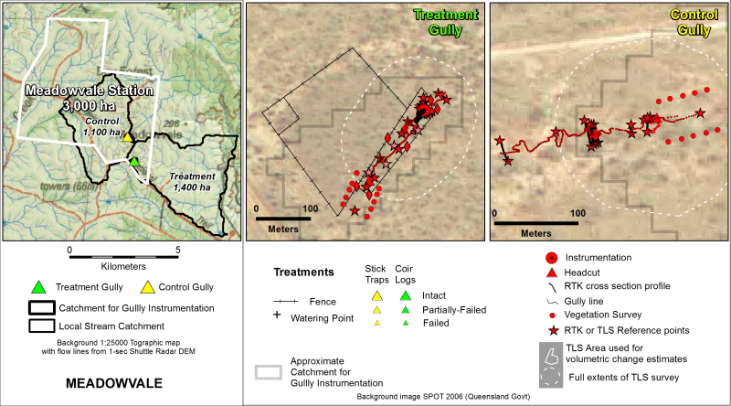
This dataset contains RTK GPS Data collected between April, 2017 and March, 2018 for 5 paired Control/Treatment gully sites being monitored as part of NESP Project 2.1.4 (Demonstration and evaluation of gully remediation on downstream water quality and agricultural production in GBR rangelands). The key question being asked is “is there measurable improvement in the erosion and water quality leaving remediated gully sites compared to sites left untreated?” The monitoring approach uses a modified BACI (Before after control impact) design. The data in presented in this metadata are part of a larger collection and are intended to be viewed in the context of the project. For further information on the project, view the parent metadata record: Demonstration and evaluation of gully remediation on downstream water quality and agricultural production in GBR rangelands (NESP TWQ 2.1.4, CSIRO). Monitoring of these sites is continuing as part of NESP TWQ Project 5.9. Any temporal extensions to this dataset will be linked to from this record. Methods: RTK (Real time kinematic) GPS system (Ashtech, ProMark 200), set with a tolerance of +/- 12mm in the horizontal plane and +/- 15mm in the vertical, was used to survey the monitored gullies. The initial location of the base station was determined using a 10-minute average. All permanent infrastructure such as survey markers, fences, and instrumentation. Gully features such as headcut rims, long sections and cross sections (at key locations such as near instrumentation) were captured. Raw GPS data files were converted to text, imported to Excel for attribute assignments, and then imported to ArcGIS for conversion to shapefile format. Format: This data collection consists of 5 zip files (one for each paired gully monitoring site). Zip files are named according to the property on which they are located. Each zip file contains two shapefiles with detailed RTK GPS survey data from either 2017 or 2018 for the Control and Treatment gullies. Survey point types include Reference markers, gully cross sections, long sections and the gully headcut. Data Dictionary: Attributes for each point include Easting (E) and Northing (N) location info (MGA94 Z55, AHD), descriptive text (Comment), horizontal accuracy (HRMS), vertical accuracy (VRMS), RTK Fix or Float status (STATUS), Number of satellites (SATS), 3D position dilution of precision (PDOP), horizontal dilution of precision (HDOP), Vertical dilution of precision (VDOP), time and date of survey point(Timestamp), and Point type (Type). More information on Dilution of Precision can be found here: https://en.wikipedia.org/wiki/Dilution_of_precision_(navigation) Point Types include REF and BASEREF - Reference markers include permanent survey markers XSREF - Cross Section Transect markers VEGREF - vegetation transect markers STRUCTREF) - Structure markers INSTRREF - location of instrumentation TLSREF - Laser scanner permanent markers gully cross sections (XS) LS - long sections RIM - headcut rim RIMNICK - headcut nickpoint Site_Code used for file names is as follows: MIV = Minnievale MV = Meadowvale MW = Mount Wickham SB = Strathbogie VP = Virginia Park <T/C> - Treatment/Control References: Bartley, Rebecca; Hawdon, Aaron; Henderson, Anne; Wilkinson, Scott; Goodwin, Nicholas; Abbott, Brett; Baker, Brett; Matthews, Mel; Boadle, David; Jarihani, Ben (Abdollah). Quantifying the effectiveness of gully remediation on off-site water quality: preliminary results from demonstration sites in the Burdekin catchment (second wet season). RRRC: NESP and CSIRO; 2018. csiro:EP184204. Data Location: This dataset is filed in the eAtlas enduring data repository at: data\nesp2\2.1.4 Gully-remediation-effectiveness

This dataset summarises the results of a survey to determine the concentration of trace metals from mine-derived pollution in marine waters and sediments across the Torres Strait during October 2016. Sampling was performed by a CSIRO team between 3 and 16 October 2016 on board the MV Eclipse. Surface water samples were collected from 21 sites using strict sampling protocols that are designed to minimise contamination (USEPA, 1996; Angel et al., 2010b). METHODS: - Sample Collection Clean powder-free vinyl gloves were worn for the handling of all sample bottles and sampling equipment, and the collection of water samples before sediment samples at any given site. Acid washed sampling bottles (0.5, 1, and 5 L), double-bagged in zip-lock bags and stored inside an esky containing ice bricks was transported on the tender to each site. The 0.5 L bottle was used to collect a sample for total mercury analysis. The 1 L bottle was used for collecting a sample for total recoverable metals analyses other than mercury, and the 5 L bottle was used for collecting a sample for filterable (dissolved) and TSS-bound metals analyses other than mercury. At every sampling site a ‘clean hands’, ‘dirty hands’ protocol was used for taking water samples. This involved the ‘clean hands’ person opening the esky, placing gloves on hands, withdrawing the 1 L sample bottle from pre-labelled zip-lock bags, placing it into an attachment on a purpose built Perspex pole sampler, uncapping the bottle and holding onto the cap. The ‘dirty hands’ person then rapidly submerged the bottle in the pole sampler to a depth of approximately 50 cm to take the sample. Each sample bottle was rinsed twice with water from the sample site by filling each bottle, capping, shaking and emptying. The 1 L bottle was used to collect water samples that were decanted into the 0.5 and 5 L bottles until they were full of sample, after which the 1 L bottle was filled a final time. The ‘clean hands’ person capped each bottle once they well filled and replaced them into the zip-lock bags in the esky. The water samples were placed into a fridge on board the MV Eclipse prior to filtration. The samples were filtered within 6 hours of sample collection. For quality control purposes, field blanks were collected at sites M, O and 8 and duplicate samples were collected at sites N, O and A. Field blanks for trace metals analysis were prepared at the designated sites by opening a 1 L bottle to the air for approximately 30 seconds followed by capping and returning to its zip-lock bag. On return to the MV Eclipse, the bottle was then filled with 1 L of deionised water. Salinity and pH were measured using an Orion Star A329 portable meter (Thermo Scientific). Sample pH was measured using a Thermo Scientific Orion Gel-Filled ROSS pH Ultra Triode Electrode (8107UWMMD) that was calibrated using pH 4.00, 7.00 and 10.00 buffers. Salinity was measured using a Thermo Scientific Orion Conductivity Cell (013010MD) that was calibrated using KCl conductivity standards. Sediment samples were collected from each site immediately after the water sampling. A combination of techniques were employed to collect the sediment samples that depended on the local water current conditions and ability of the corer to penetrate the sediment. Firstly, a gravity core sampler was deployed from the Eclipse, which collected up to 12 cm deep sediment within pre-loaded plastic core tubes. If this was unsuccessful divers took hand cores of up to 7 cm depth by diving to the sea bed. The core tubes were capped with plastic stoppers and wherever possible, returned to the surface in an upright position. If the substrate was too hard for hand coring, the divers took a grab of loose sediment samples by hand inside 250 mL polycarbonate vials. The core tubes were withdrawn from the corer on-board the MV Eclipse, placed into zip-lock bags, and placed inside a freezer until frozen. The cores were then sectioned by allowing a core to partially thaw so that the sediment core could be extruded with a plastic plunger, before cutting into sections (typically 1-2 cm length) with a plastic blade. The core sections were placed into zip-lock bags and stored frozen for transport to the Lucas Heights laboratories. The contents of some of the shorter unconsolidated sediment cores became mixed, in which case the entire core was treated as a single sample rather than sub-sectioning. Triplicate cores/sediment grabs were generally taken at each site in order to assess sampling heterogeneity. - Water sample processing Water samples for analysis of trace metals were vacuum filtered through acid-washed 0.45 µm Millipore membrane filters using an acid washed polycarbonate filtration apparatus (Sartorius). The filtration assemblies were further cleaned before processing each sample by first filtering a 100 mL volume of 10% v/v nitric acid solution followed by two 150 mL volumes of deionised water, and finally, a 50 mL volume of sample. For each volume of these solutions the filtration rig was held on an angle and rotated both before and after filtration so that the solutions came into contact with all surfaces of the top and bottom compartments of the apparatus to ensure rigorous rinsing / pre-treatment was achieved. The 50 mL aliquot of sample used to pre-clean the filtration rig was poured into the 1 L acid washed Nalgene filtrate receiving bottle, shaken to pre-treat the bottle, and discarded to waste. The sample was then filtered and the filtrate transferred into the receiving bottle. Between 4-6 L of each sample filtrate was retained for analysis. Filtrates were then preserved by addition of 2 mL/L of concentrated nitric acid (Merck Tracepur). For the field blanks, approximately half of the 1L sample was filtered and preserved. The remaining 500 mL was acidified and retained for subsequent analysis. The difference between the filtered and unfiltered field blanks gave an indication if filtration resulted in contamination. Suspended sediment samples for total suspended sediment (TSS) and TSS-bound metals analyses were acquired by filtering known volumes of water through pre-weighed 0.45 µm membrane filters (Millipore). The filters were rinsed with 10% nitric acid before use and each sample was filtered using the filtration procedure described above. After the sample was filtered and the filtrate removed, the upper compartment of the filtration apparatus and the filter were rinsed with approximately 20 mL of deionised water to remove any salt. The filters were placed into acid-washed plastic Petri slides and stored frozen. The filters were transferred to the CSIRO Lucas Heights laboratories, after which they were oven-dried at 60oC, cooled to room temperature in a desiccator, and weighed. This procedure was repeated three times to ensure the mass was consistent, after which, the filters were stored at room temperature until total recoverable (TR) metals analysis was performed. The TSS concentration (mg/L) of the water samples was calculated using the difference in the mass of the filter before and after filtration divided by the volume of sample filtered. - Analysis of dissolved metals Dissolved Cd, Co, Cu, Ni, Pb and Zn in filtered samples were analysed by complexation and solvent extraction prior followed by quantitation of the pre-concentrated metals by ICPMS. The extraction procedure allowed the pre-concentration of metals by a factor of 25, thus allowing more accurate quantification. A dithiocarbamate complexation/solvent extraction method based on the procedure described by Magnusson and Westerlund (1981) was employed. The major differences were the use of a combined sodium bicarbonate buffer/ammonium pyrrolidine dithiocarbamate reagent (Apte and Gunn, 1987) and 1,1,1-trichloroethane as the extraction solvent in place of Freon. In brief, sample aliquots (250 mL) were buffered to pH 5 by the addition of the combined reagent and extracted into two 10-mL portions of triple-distilled trichloroethane. The extracts were combined and the metals back-extracted into 1 mL of concentrated nitric acid (Merck Tracepur). The back extracts were diluted to a final volume of 10 mL by addition of deionised water and analysed by inductively coupled plasma-mass spectrometry (ICPMS) (Agilent, 7500CE) using the instrument operating conditions recommended by the manufacturer. For quality control purposes a portion of the certified reference seawater NASS-6 (National Research Council (NRC), Canada) CRM was analysed in every sample batch. Dissolved aluminium and iron concentrations were measured directly on portions of acidified filtered waters by ICP-AES (Varian730 ES) using matrix-matched standards. The concentrations of dissolved chromium were measured directly by ICP-MS (Agilent 7500CE ) following three-fold dilution with deionised water and calibration against matrix-matched standards. The concentration of dissolved arsenic in the filtered samples was measured by hydride generation atomic absorption spectrometry (HG-AAS), using procedures based on the standard methods described by APHA (1998). Samples were first digested by addition of potassium persulfate (1% m/v final concentration) and heating to 120°C for 30 min in an autoclave. Hydrochloric acid, (3 M final concentration) was then added to the samples. Pentavalent arsenic was then pre-reduced to arsenic (III) by addition of potassium iodide (1% (m/v) final concentration) and ascorbic acid (0.2% (m/v) final concentration) and left standing for at least 30 min at room temperature prior to analysis. Arsenic concentrations were then measured by HG-AAS using a Varian VGA system operated under standard conditions recommended by the manufacturer. Arsenic (III) in solution was reduced to arsine by reduction with sodium borohydride, which was stripped from solution with argon gas into a silica tube, electrically heated at 925°C. Heating converted arsine into arsenic vapour, which was quantified by atomic absorption spectrometry. For quality control purposes a portion of the certified reference seawater NASS-6 (National Research Council (NRC), Canada) CRM was analysed in every sample batch. DOC was measured on aliquots of filtered samples collected during the June 2018 survey using a Shimadzu TOC-LCSH Total Organic Carbon Analyser using the procedures recommended by the manufacturer. - Analysis of metals bound to total suspended solids (TSS) and benthic sediment The TSS and benthic sediment was digested in pre-cleaned Teflon digestion vessels using aqua-regia digestions in a microwave-assisted reaction system (MARS). The membrane filters containing the suspended sediments or known quantities of dry benthic sediment were transferred into the MARS digestion vessels and subjected to pressurised digestion. The method involved adding 2.5 mL of concentrated nitric acid (Tracepur, Merck) and 7.5 mL of concentrated hydrochloric acid (Tracepur, Merck) to each digestion vessel and heating at high pressure in a MARS digestion system for 90 minutes. Once cool, the digest vessels were vented followed by dilution of the digest to a final volume of 40 mL using deionised water. The masses of the empty vessel, the vessel plus sample, and the vessel plus sample and acid mixture before and after heating were recorded to allow calculation of a dilution factor used in the determination of metal concentrations in the initial undiluted sample. For quality control purposes, portions of the certified reference sediments ERM-CC018 (IRMM) and PACS-3 (NRC Canada) were analysed in each sample batch. Format: This dataset consists of multiple Comma Separated Value (CSV) tables containing the data provided by the project team. Data Location: This dataset is filed in the eAtlas enduring data repository at: data\NESP-TWQ-2\2.2.2_TS-mine-pollution

An updated version of this dataset is available at https://eatlas.org.au/data/uuid/38b496a3-3fba-42e7-b904-902f68040c85 Key Gully monitoring localities (headcuts and monitoring instrumentation) and outlines of the properties within which they are located. The data in presented in this metadata are part of a larger collection and are intended to be viewed in the context of the project. For further information on the project, view the parent metadata record: Demonstration and evaluation of gully remediation on downstream water quality and agricultural production in GBR rangelands (NESP TWQ 2.1.4, CSIRO) Methods: Key Gully Localities were extracted from the 2017 or 2018 RTK GPS surveys for each gully site (see Site_Configuration_and_Survey). Property Boundaries were generated by extracting polygons from the 2016 Digital Cadastre Database (DCDB) and simplifying to a single polygon. Area in hectares was calculated and appended to polygon attributes. KMZ’s are exported version of the original ArcGIS shapefiles Format: This data collection consists of two shapefiles (zipped) and two equivalent KMZ files with the following names: NESP_Gully_Key_localities Key gully localities include the RTK GP location of the instrumentation and the RTK GPS location of the nickpoint in the gully headcut rim. NESP_Gully_Property_Boundaries Boundaries for the properties on which the paired control/treatment gullies are located. Data Dictionary: Attributes for Property_Boundaries.shp include property NAME and the area in hectares (AREA_HA). Attributes for Key Locations include X,Y (MGA94 Z55) and Z (AHD) Timestamp associated when RTK surveyed Type- HEADCUT, INSTR Survey – type of survey and year, APPROX is best guess from Lidar or GoogleEarth Site_Code – short form code for sites where MIV = Minnievale MV = Meadowvale MW = Mount Wickham SB = Strathbogie VP = Virginia Park <T/C> - Treatment/Control Property – Full name of property Treat_type – Treatment or control References: Bartley, Rebecca; Hawdon, Aaron; Henderson, Anne; Wilkinson, Scott; Goodwin, Nicholas; Abbott, Brett; Baker, Brett; Matthews, Mel; Boadle, David; Jarihani, Ben (Abdollah). (2018) Quantifying the effectiveness of gully remediation on off-site water quality: preliminary results from demonstration sites in the Burdekin catchment (second wet season). RRRC: NESP and CSIRO. csiro:EP184204. Data Location: This dataset is filed in the eAtlas enduring data repository at: data\NESP2\2.1.4_Gully-remediation-effectiveness